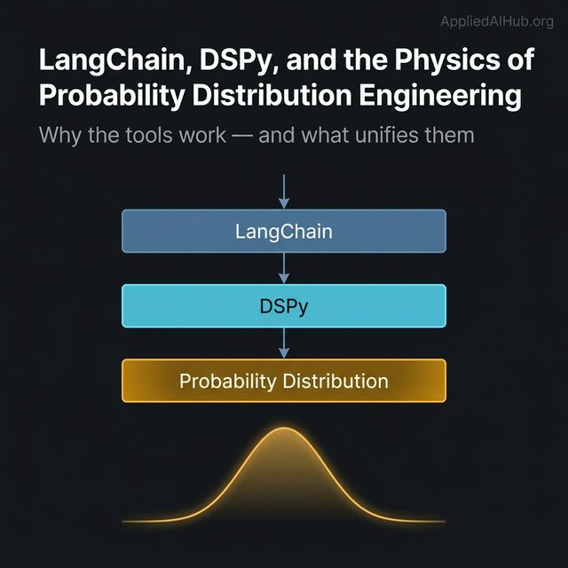
LangChain, DSPy, and the Physics of Probability Engineering
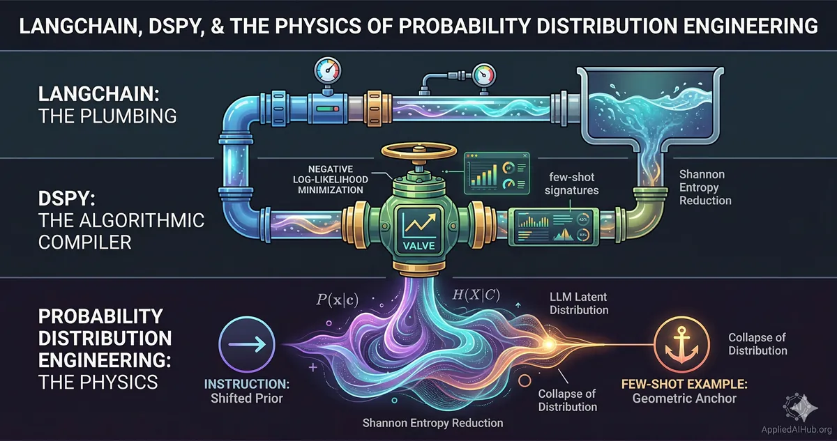
- LangChain solves the external plumbing problem — how to connect components — but says nothing about the reliability of what flows through those connections.
- DSPy automates the search for high-quality prompts through gradient-free optimization, but the mathematical goal it pursues is still minimizing the negative log-likelihood of correct outputs.
- Both tools are implementations of the same underlying physics: the manipulation of a high-dimensional probability distribution over a latent space.
A thread on r/PromptEngineering last week opened with a genuinely sharp question: “Is ‘probability distribution engineering’ just a fancy way of saying ‘be more specific’? And isn’t that just DSPy running automatically?”
Both challenges are worth taking seriously, because the person asking them isn’t wrong about the surface-level overlap. They’re wrong about what layer of abstraction they’re operating on.
Here’s the more productive framing: LangChain, DSPy, and “probability distribution engineering” are not competing answers to the same question. They are answers to questions at three completely different levels of the stack. Conflating them is like asking whether a building’s water pressure problem is best solved by changing the pipes, recalibrating the pressure regulator, or understanding fluid dynamics. The correct answer depends entirely on the problem — and you cannot make good decisions at any level without understanding the level below it.
The water metaphor is deliberate. Keep it in mind.
LangChain: Industrial-Grade Plumbing
LangChain’s core value proposition is composability. It provides standardized interfaces — chains, agents, retrievers, memory stores, tool callers — that allow you to connect heterogeneous components without writing bespoke integration code for every combination.
Want to connect a vector database query to a summarization model, pass the result to a structured output parser, and log the whole thing to a trace store? LangChain gives you that scaffolding. It solves a real problem: LLM-powered applications involve many moving parts, and gluing them together manually is tedious, fragile, and hard to test.
What LangChain does not solve — and was never designed to solve — is what happens inside the LLM itself.
The framework tells you how to connect the pipes. It says nothing about the pressure, the viscosity, or the quality of whatever is flowing through them. A RAG pipeline built in LangChain can still hallucinate confidently if the retriever returns low-relevance chunks and the prompt provides no mechanism to suppress fabrication. The framework executed perfectly. The probability distribution of the LLM’s output was still a disaster.
Author’s Comments: The “Chain Succeeds, Output Fails” Pattern
In production, the most insidious LangChain failures are the ones where everything runs without exception and the output is still wrong. No error. No trace. Just semantically incorrect content delivered with full confidence. When I see this pattern, my first question is never “did the chain fail?” — it’s “did the distribution drift?” Usually, someone changed the upstream data, and the prompt was never designed to handle the new distribution of inputs. I’ve seen teams spend days debugging LangChain configuration when the actual fix was a three-line prompt constraint.
The scaffolding metaphor is accurate: LangChain organizes the construction site. It makes the work possible at scale. But you can build a structurally unsound building on a perfectly organized construction site.
DSPy: An Algorithmic Compiler for Prompts
Stanford’s DSPy (Declarative Self-improving Language Programs) makes a different kind of bet. Instead of asking you to hand-write and tweak prompt strings, it lets you declare the shape of what you want through Signatures: a typed specification of inputs and outputs.
class SentimentClassifier(dspy.Signature):
    """Classify the sentiment of a product review."""
    review: str = dspy.InputField()
    sentiment: Literal["positive", "negative", "neutral"] = dspy.OutputField()
The optimizer (originally called a Teleprompter, now just an optimizer) then uses your labeled examples and a metric function to automatically search for the prompt — including any few-shot demonstrations — that best achieves your target output.
This directly addresses one of the most expensive problems in LLM engineering: ad-hoc prompt hacking. The standard workflow without DSPy looks like this: write a prompt, test it on a few examples, notice it fails on edge cases, rewrite it, test again, repeat until you get bored or ship. DSPy replaces that loop with a principled, reproducible optimization pass.
The Reddit commenter who said “isn’t this just DSPy?” was gesturing at something real: DSPy does, in fact, automate the search through prompt space for better-performing configurations. But knowing what DSPy does is not the same as knowing why it works, or why it sometimes fails, or how to set up your metric function so that the optimizer converges on something meaningful rather than a prompt that games your validation set.
The Mathematical Goal DSPy Is Actually Pursuing
When DSPy’s optimizer evaluates a candidate prompt , it is — at the mathematical level — measuring the conditional probability that prompt generates the correct output given input :
This is the negative log-likelihood. Minimizing it is minimizing surprise — maximizing the probability the model assigns to the correct answer. DSPy automates the gradient-free search over the discrete prompt space to minimize this loss on your examples.
That is elegant engineering. But it is also a black box optimization. DSPy tells you which prompt worked best on your validation set. It does not tell you why the winning prompt distributes probability mass more favorably — what structural property of that prompt text creates sharper, lower-entropy predictions from the model. That explanation lives one level deeper.
Probability Distribution Engineering: The Fluid Dynamics Layer
Here is the underlying physical reality that both tools are operating on, whether or not they make it explicit.
An LLM is not a function that maps an input string to an output string. It is a machine that, at each generation step, outputs a full probability distribution over its entire vocabulary. The next token is sampled from that distribution. Then the distribution is recomputed. Then the next token is sampled. The output you receive is a single path through an astronomically large probability tree.
Your prompt is the initial boundary condition that shapes every distribution in that tree.
As I established in The Probability Theory of Prompts, a vague prompt places the model in a state of maximum entropy. The probability mass is spread thin across an enormous vocabulary. The model is, in the precise information-theoretic sense of the word, guessing. The conditional entropy is high, and the output is correspondingly variable and unreliable.
Good prompting is entropy reduction. Every meaningful constraint you add — a role, a format requirement, a concrete specification of who the output is for — collapses the distribution toward a narrower, more predictable region of the latent space.
Why Few-Shot Examples Are More Efficient Than Instructions
This distinction has practical teeth. Consider two strategies for communicating the same requirement:
Strategy A (Instruction): “Write in a professional but concise tone, avoiding passive voice, and keep your sentences under 20 words.”
Strategy B (Demonstration): A single high-quality example of output that embodies all of those properties.
Both strategies shift the probability distribution toward your target. But Strategy B is typically more efficient per token. Why?
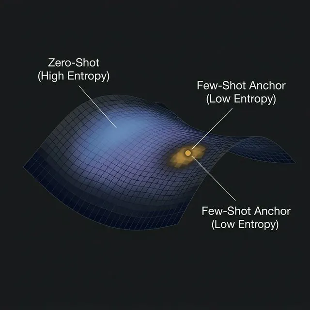
Instructions operate through semantic parsing — the model must interpret the instruction, map it to abstract style properties, and then execute those properties. Each step in that chain introduces variance. Demonstrations operate through a different mechanism: they place geometric anchors on the model’s latent manifold.
The model’s internal representations live in a high-dimensional geometric space. Your few-shot example is a specific point on that manifold. The model’s nearest-neighbor intuition — learned through billions of training steps — causes it to generate output that is geometrically close to that anchor point. This is not a metaphor. It is a consequence of how the attention mechanism computes similarity in embedding space.
This is the mathematical reason zero-shot vs. few-shot prompting is not just a pedagogical distinction. The two techniques exert fundamentally different types of geometric constraint on the distribution. Instructions shift the model’s prior. Examples constrain the manifold neighborhood it samples from.
Entropy, Constraints, and the Right Vocabulary
The formal definition of Shannon entropy applied to a model’s output distribution at step is:
A high means the distribution is flat: many tokens are roughly equally plausible. A low means the distribution is sharp: one or a small number of tokens dominate. Your goal as a prompt engineer is to construct a context that minimizes for every step of generation that matters.
Every technique in the standard prompt engineering toolkit maps directly to this goal:
- Role prompting projects the model’s distribution onto a domain-specific submanifold, eliminating probability mass from irrelevant domains.
- Format constraints (e.g., “Output valid JSON only”) force terminal tokens like
{and}toward probability 1, collapsing the distribution around structured output. - Negative constraints (“Do not include explanations”) explicitly zero out probability mass from an entire class of tokens.
- Chain-of-thought elicitation restructures the generation sequence so that intermediate reasoning tokens provide additional boundary conditions for subsequent token distributions.
These are not stylistic preferences. They are operations on a probability distribution.
How the Three Layers Relate
The water analogy completes itself here.
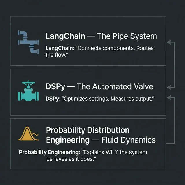
LangChain is the pipe system. It determines what flows where, in what order, and how components connect. A well-designed pipe system is necessary for any serious application. But the pipe system is indifferent to whether the water is clean.
DSPy is the electronically controlled pressure valve. It knows — through measurement and optimization — how to adjust its settings to achieve a target flow rate at the output. It is empirical and automated. It does not need to know the fluid dynamics to find a good setting.
Probability distribution engineering is fluid dynamics itself. It explains why certain pipe configurations create turbulence, why certain valve settings cause cavitation, and why the system behaves differently under different input pressures. It is the underlying physics that makes sense of everything above it.
You do not need fluid dynamics to be a plumber. But when the system behaves unexpectedly — and it will — fluid dynamics is the only framework that lets you reason about why.
Why LangChain Chains Fail: Distribution Drift
Consider a LangChain RAG pipeline that worked flawlessly for three months and then began producing degraded output with no code changes. The usual culprits:
- The upstream document corpus changed structure or vocabulary.
- The embedding model’s retrieval behavior shifted the quality of chunks being returned.
- The real-world distribution of user queries drifted away from the distribution the prompt was implicitly calibrated for.
In every case, the chain itself is functioning correctly. What failed is the probability distribution at the LLM’s input boundary. The prompt was designed for one input distribution and is now receiving another. The effective constraints it provides no longer produce sharp, reliable output distributions.
Debugging this by rewriting the prompt by feel is expensive and unpredictable. Debugging it by asking “which constraint degraded, and why did the input distribution shift?” is faster and produces a fix that generalizes.
Why DSPy Optimizations Sometimes Overfit
DSPy’s optimizer is powerful, but it minimizes loss on a validation set, not on a probability distribution. If your validation examples don’t cover the full range of your real input distribution, the winning prompt is overfit to a narrow corridor of the latent space. In production, inputs that fall outside that corridor encounter a prompt that has not learned to constrain the distribution for them.
Understanding this is not a criticism of DSPy. It is a reminder that the optimizer is maximizing a proxy metric, and the underlying target — a prompt that reliably collapses the output distribution to correct answers across the full input manifold — is a geometric property that no finite validation set fully specifies.
Practical Consequences of This View
Debugging Unstable Output
When AI output is inconsistent across runs or degrades over time, the productive diagnostic question is not “what should I add to the prompt?” It is: “which dimension of the probability space has become under-constrained?”
This reframe almost always narrows the search. If outputs are inconsistently formatted, the format constraint is insufficient. If outputs are factually variable, the factual grounding (context injection) is insufficient. If outputs are tonally inconsistent, the role or persona constraint is too loose. Each symptom maps to a specific type of distributional slack.
Hard vs. Soft Constraint Architecture
When designing pipelines, two fundamentally different classes of constraint are available:
Hard projections operate at the infrastructure level. JSON mode, grammar-constrained decoding, and function calling schemas constrain token sampling directly — they force probability mass to zero for tokens that would violate the structure. This is the most reliable form of entropy reduction, because it operates beneath the prompt layer.
Soft guidance operates through the prompt itself. Role descriptions, instructions, few-shot examples, and constraint language shift the distribution without enforcing hard boundaries. These are more flexible but introduce variance.
The professional approach is to use hard projections whenever your output requirement can be formally specified, and treat soft guidance as complementary rather than primary.
This is also where understanding the distribution has a practical cost advantage. A Prompt Scaffold is useful here precisely because it forces you to specify format and constraints in dedicated fields — preventing the most common failure mode, where constraint language gets buried inside a long task description and loses its distributional impact. And because Prompt Scaffold runs entirely in-browser with no backend, there is no API call and no token overhead during the design phase itself. You can iterate on constraint architecture — roles, negative constraints, format rules — until the structure is sound, then paste the resulting prompt into any model you choose. The insight that reliable outputs come from constraint precision rather than model size means you get more consistent results for less cost, without depending on any particular provider.
Predicting Where the Field Goes
As models scale further and instruction-following improves, the naive interpretation of this trend is that prompting becomes less important — the model is smart enough to figure it out. This misunderstands the problem.
Improved instruction-following means each unit of constraint you provide collapses more distribution than it did before. The model becomes more sensitive to constraints, not less dependent on them. What changes is that imprecise constraints start to matter more, not less — a vague role instruction that a weaker model approximately honored is now taken more literally, for better or worse.
The engineers who understand the distribution will know how to exploit this. The engineers who are guessing will find their prompts becoming less reliable as models become more capable, not more.
A Note to the Reddit Skeptics
To the commenter who asked whether this is just “be more specific, but fancier”: partially yes. But “be more specific” is a heuristic with no explanatory power. It tells you what to do without telling you why it works or when it fails. The probability framework gives you a principled account of the mechanism, which means you can generalize it, debug with it, and reason about edge cases.
To the commenter who asked “isn’t this just DSPy?”: DSPy is an automated search algorithm operating over this space. Knowing what DSPy is doing — minimizing negative log-likelihood on a validation set by searching discrete prompt space — tells you exactly when to trust its output and when to be skeptical. That knowledge comes from understanding the distribution, not from using the tool.
The tools are useful. The physics is why the tools work.
Related reading:
- The Probability Theory of Prompts — The mathematical foundation: how prompts function as projection operators on a high-dimensional probability space.
- Zero-Shot vs. Few-Shot Prompting — Why examples and instructions exert geometrically different constraints on the output distribution.
- Chain-of-Thought Prompting Explained — How generating intermediate reasoning tokens restructures the generation sequence and changes which distributions the model samples from.
- The RTGO Prompt Framework — A practical implementation of multi-constraint prompting through the lens of Measure Theory parameters.
Support Applied AI Hub
I spend a lot of time researching and writing these deep dives to keep them high-quality. If you found this insight helpful, consider buying me a coffee! It keeps the research going. Cheers!

This site uses no tracking cookies or intrusive ads. Your support helps keep it that way.